Error estimation in differential photometry

It is possible, if one knows in detail many of the electronic characteristics of one's CCD camera, to estimate a priori the sorts of errors that one may expect from differential photometry. This is by no means a small task, and may well be beyond the technical ability (and interest) and time constraints of many observers. This is in no way meant as a put-down of this method; rather, that it is involved and perhaps more so than many would wish to accept.

As mentioned on the main Photometry page, one may use a check star (and preferably more than one) not only to assess the stability of the comparison star, but also as a means of estimating the error of the data on the variable star. If the check star, K, is of similar brightness to the variable star, V, then the statistics of C-K will be similar to the statistics of C-V.

If K is fainter than V, the C-K error will over-estimate the C-V error.

If K is brighter than V, the C-K error will underestimate the C-V error.

If the only possible option is to measure a single K star only, try to choose one that is around the average brightness of V. This way, C-K errors will provide an "average" indication of the expected errors in C-V.

Now, if one can choose and measure a whole swarm of K stars, which range from fainter than, to much tha same as, and to brighter than V, one may estimate the errors for any value of C-V. The more stars the merrier; perhaps around six as a minimum, and a dozen or so would be good.

For a data run on a particular field, obtain the differential magnitudes for the variable star and for all your selected check stars. You will then have a set of differential magnitudes vs. time (i.e. time series) for C-V and C-K1, C-K2, C-K3, etc. For each of these time series, calculate the standard deviation of the time series, and its average magnitude. If, as an example, you have ten check stars and one variable, you will end up with 11 pairs of numbers of the form

(ave. magnitude, standard deviation)

to be considered as (x,y) pairs for plotting on a graph. Plot them out (using a spreadsheet or other suitable software), and fit an exponential curve to the (x,y)-pairs for the C-K values only (do not include the C-V pair in this step- treat it strictly as a separate series on the graph). The software should be able to tell you the equation that was used to fit the curve to the points.

This equation will allow you to estimate a y-value (i.e. scatter, to be interpreted as expected error) for any x-value (i.e. differential magnitude) for the conditions that prevailed at the time of that particular observing run. Use the software to generate an expected error for each C-V point, and then use this as the size of the y-error-bars on a plot of the C-V time series. Each of these errors will be appropriate to the magnitude of V at that time.

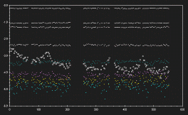
Diff. mag. vs. time (minutes) : about 9 hours of C-V and C-K data for the field of EUVE J2115-58.6 on the night of 27-28/7/1997. Check stars are crosses of various colours, and the variable is denoted by a circle. It is evident that the scatter in the data increases as one goes to fainter stars. It also is clear that the V star varies considerably in overall brightness, so that a single error estimate would not be accurate for all the C-V values shown.

Scatter vs. ave. diff. magnitude : a plot of standard deviation (scatter) vs. average differential magnitude for the time series shown in the first diagram. An exponential fit to the C-K pairs is shown, along with the equation of the fit. K star value are shown as crosses; the variable is denoted by a circle. Note that the V star is highly variable- it lies well above the trend for expected errors due to measurement errors alone, and is therefore significantly intrinsically variable.

Diff. mag. vs. time (minutes) : C-V data with error bars added. Note that the size of the error changes with the brightness of the V star; larger when V is fainter, smaller when it is brighter.

This method makes no assumptions about the characteristics of the CCD camera, and as it uses the actual data to estimate the error, it will reflect the actual observing conditions prevailing during the observing run. Nights which are photometrically poor (even for the relavtively forgiving nature of differential photometry), will show larger scatter than those nights which are of high quality. This will show up in the size of the errors allocated to the C-V points, and will alert the observer to data which may be too poor to use. Also, changing photometric quality during a night will, quite likely, be readily apparent as an increse or decrease in scatter of the C-K data during the night.

It may by chance happen that one of the K stars will be variable. This may be shown by a continued habit of it appearing above the general trend of your scatter points- in which case, you may have discovered a new (but possibly quite faint) variable star.

A photometric reduction package which allows the choosing of multiple K stars will allow this sort of reduction to be undertaken with minimal extra effort on the part of the observer. If such a method is employed, one will have a thorough idea of the errors in your data for each data run, a good long-term check of the stability of C, a sample of stars to check for new variables, and, over time, a good guide to the sort of accuracy attainable with your equipment and the general stability of your observing site with regard to photometric quality.